The Key-Ring Problem
You find a key-ring on the ground. $N$ keys, one door, no labels. What do you do? You try every last one. In the worst case, you try all $N$. On average, $\frac{N}{2}$. No cleverness saves you here; any classical strategy for searching an unstructured collection requires $O(N)$ tries.
This is the problem of searching an unsorted database. Given $N$ items, find the one that satisfies some property. Classically, there is nothing faster than brute force.
But what if the keys existed in a kind of superposition – all being tried at once, in a space where interference could amplify the correct answer and suppress the wrong ones? In 1996, Lov Grover showed that a quantum computer can find the needle in the haystack using only $O(\sqrt{N})$ queries. For a million items, that is 1,000 queries instead of 1,000,000. In the same paper, he proved this is the best any quantum algorithm can do.
Herein we build your understanding of Grover’s algorithm from the ground up. If you have taken Calculus 1 through 3 and have seen matrices and dot products, you have all the prerequisites. Everything else, we build together. By the end, you will understand not only why the algorithm works, but why it must be stopped at the right moment – a property that has no classical analogue and is, frankly, one of the strangest things in all of computer science.
The Calculus Bridge: Rotation as Repeated Small Kicks
Before we touch any quantum mechanics, let us build the geometric intuition that makes the whole thing click. No qubits required. Just calculus.
Euler’s Method Recap
In Calculus you learned to solve differential equations like $\frac{dy}{dx} = f(x, y)$ numerically using Euler’s method: start at a known point, take a small step in the direction of the derivative, repeat.
Each step is an approximation. The key insight – and this is worth pausing on – is:
- Too few steps: you have not reached the target yet.
- Just right: you land close to the true solution.
- Too many steps: you overshoot and diverge away from the answer.
The step size matters. If each step is $h$, then after $k$ steps you have traveled approximately $kh$ total. Overshoot is not a bug in your code; it is a fundamental property of discrete approximations to continuous problems.
Rotation on a Circle
Now consider a different scenario: you have a vector starting nearly horizontal, and you want to rotate it to point straight up (vertical). Suppose each “kick” rotates the vector by a small angle $2\theta$.
After $k$ kicks, the vector has rotated by $2k\theta$ total. You want the total rotation to be $\frac{\pi}{2}$ (a quarter turn, from horizontal to vertical):
\[2k\theta \approx \frac{\pi}{2} \implies k \approx \frac{\pi}{4\theta}\]If the angle $\theta$ is small – say $\theta \approx \frac{1}{\sqrt{N}}$ – then you need about $\frac{\pi}{4}\sqrt{N}$ kicks. Now here is where it gets wild: keep kicking past that sweet spot and the vector rotates past vertical, pointing away from the target. The alignment gets worse the more work you do.
This is exactly what Grover’s algorithm does. Each iteration is a small angular kick, rotating a quantum state vector toward the solution. The “vector pointing up” represents having found the answer. And just like Euler’s method, if you take too many kicks, the vector overshoots and the probability of finding the answer actually decreases.
We will return to this analogy in full force once we have the quantum vocabulary to make it precise. Keep this picture in your head: a vector on a circle, being kicked toward vertical, one small rotation at a time.
Quantum Vocabulary
This section introduces the mathematical language of quantum computing. Each concept is motivated by why you need it, defined precisely, and connected back to mathematics you already know from Calc 1-3. If something feels dense, keep reading – the payoff is in the algorithm itself, and these tools will serve you well beyond this post.
Bra-Ket Notation
Why you need this: Physicists write vectors differently than mathematicians. Since quantum computing grew out of physics, we inherit their notation. It is just a shorthand for things you already know. Do not let the angle brackets intimidate you.
A ket $\lvert \psi \rangle$ is simply a column vector:
\[\lvert \psi \rangle = \begin{pmatrix} a_1 \\ a_2 \\ \vdots \\ a_n \end{pmatrix}\]where each $a_i$ is a complex number called a probability amplitude.
A bra $\langle \psi \rvert$ is the conjugate transpose (take the transpose, then complex-conjugate every entry):
\[\langle \psi \rvert = \begin{pmatrix} a_1^* & a_2^* & \cdots & a_n^* \end{pmatrix}\]The inner product (the “bra-ket,” get it?) of two states is the generalized dot product you know from Calc 3:
\[\langle \phi \mid \psi \rangle = \sum_{i} b_i^* \, a_i\]This is a single complex number. When $\langle \phi \mid \psi \rangle = 0$, the states are orthogonal – perpendicular, in the language you already speak.
Normalization: A valid quantum state must satisfy $\langle \psi \mid \psi \rangle = 1$. The vector has unit length. The probability of measuring outcome $i$ is $\lvert a_i \rvert^2$, and these must sum to 1. If this reminds you of the constraint that a unit vector in $\mathbb{R}^n$ satisfies $\sum x_i^2 = 1$, good – it is the same idea, extended to complex numbers.
The Computational Basis
The simplest quantum states for a single qubit are:
\[\lvert 0 \rangle = \begin{pmatrix} 1 \\ 0 \end{pmatrix}, \quad \lvert 1 \rangle = \begin{pmatrix} 0 \\ 1 \end{pmatrix}\]Any single-qubit state can be written as a linear combination: $\lvert \psi \rangle = \alpha \lvert 0 \rangle + \beta \lvert 1 \rangle$ with $\lvert \alpha \rvert^2 + \lvert \beta \rvert^2 = 1$. That is the whole game. Superposition is just linear combination with a normalization constraint.
Unitary Matrices: Rotations That Preserve Length
Why you need this: Quantum operations must preserve the total probability of 1. The matrices that preserve vector length are exactly the unitary matrices – the complex generalization of the rotation matrices you know from Calc 3.
Recall that a rotation matrix $R$ in $\mathbb{R}^2$ preserves length: $\lVert Rv \rVert = \lVert v \rVert$. The defining property is $R^T R = I$. Unitary matrices are the same idea, but for complex vectors: transpose becomes conjugate transpose.
A matrix $U$ is unitary if:
\[U^\dagger U = I\]where $U^\dagger$ denotes the conjugate transpose and $I$ is the identity matrix.
Key properties:
- The columns of $U$ form an orthonormal basis.
- $\lvert \det(U) \rvert = 1$.
- Every quantum gate is a unitary matrix. This guarantees that quantum computation is reversible and probability-preserving.
import numpy as np

# A 2x2 unitary matrix
U = np.array([[1/np.sqrt(2), -1j/np.sqrt(2)],
              [1j/np.sqrt(2),  1/np.sqrt(2)]])

# Verify: U dagger U = I
print(np.allclose(U.conj().T @ U, np.eye(2)))  # True
Hermitian Matrices: The Matrices of Measurement
Why you need this: So why should you care about Hermitian matrices? Because in quantum mechanics, anything you can physically measure – energy, position, momentum – is represented by a Hermitian matrix. Their eigenvalues are always real numbers, which makes sense because measurement results are real. That is not a coincidence; it is the reason physicists use them.
A matrix $A$ is Hermitian (also called self-adjoint) if:
\[A = A^\dagger\]It equals its own conjugate transpose. Equivalently, $A_{ij} = A_{ji}^*$ – each entry above the diagonal is the complex conjugate of the entry below.
Key properties:
- All eigenvalues are real.
- Eigenvectors for distinct eigenvalues are orthogonal.
- A Hermitian matrix can always be diagonalized by a unitary matrix (the spectral theorem).
Example: The matrix $\begin{pmatrix} 2 & 1-i \ 1+i & 3 \end{pmatrix}$ is Hermitian. Swap rows and columns, conjugate, and you get the same matrix back. Check it yourself – it takes ten seconds.
The Hamiltonian: The Energy Operator
Why you need this: The Hamiltonian tells a quantum system how to evolve in time. It is the bridge between quantum mechanics and the differential equations you studied in Calculus. If you understood $\frac{dy}{dx} = ky$ and its solution $y = y_0 e^{kx}$, you already have the intuition.
The Hamiltonian $\hat{H}$ is a Hermitian matrix representing the total energy of a quantum system. The fundamental equation governing quantum time evolution is the Schrodinger equation:
\[i\hbar \frac{d}{dt} \lvert \psi(t) \rangle = \hat{H} \lvert \psi(t) \rangle\]This is a first-order linear ODE! Its solution, when $\hat{H}$ is time-independent, is:
\[\lvert \psi(t) \rangle = e^{-i\hat{H}t/\hbar} \lvert \psi(0) \rangle\]The operator $e^{-i\hat{H}t/\hbar}$ is unitary (preserves probabilities), and it acts as a rotation in the state space. This is the deep connection: time evolution in quantum mechanics is rotation, driven by the Hamiltonian. When we say “each Grover iteration rotates the state by $2\theta$,” we are implicitly standing in this framework.
We will not use the Hamiltonian directly in Grover’s algorithm, but the intuition that quantum operations are rotations is the Hamiltonian picture at work, and it will serve you well in everything quantum from here forward.
Notation warning: Two critical concepts, one letter. The Hamiltonian is often written $\hat{H}$ or $\mathcal{H}$. This is different from the Hadamard gate $H$ (no hat), introduced next. Physicists are a generous people, but nomenclature is not their gift. Context will always make clear which is meant.
The Hadamard Gate: The Coin-Flip Operator
Why you need this: To search all possibilities at once, we need a state that is an equal superposition of every possible answer. The Hadamard gate creates exactly this – it is the quantum equivalent of flipping a perfectly fair coin.
The Hadamard gate $H$ is the $2 \times 2$ unitary matrix:
\[H = \frac{1}{\sqrt{2}} \begin{pmatrix} 1 & 1 \\ 1 & -1 \end{pmatrix}\]Its action on the computational basis states:
\[H\lvert 0 \rangle = \frac{\lvert 0 \rangle + \lvert 1 \rangle}{\sqrt{2}}, \qquad H\lvert 1 \rangle = \frac{\lvert 0 \rangle - \lvert 1 \rangle}{\sqrt{2}}\]Applied to $n$ qubits all starting in $\lvert 0 \rangle$, the tensor product $H^{\otimes n}\lvert 0 \rangle^{\otimes n}$ creates a uniform superposition over all $N = 2^n$ basis states:
\[\lvert \phi \rangle = H^{\otimes n}\lvert 0 \rangle^{\otimes n} = \frac{1}{\sqrt{N}} \sum_{x=0}^{N-1} \lvert x \rangle\]Every key is now being tried with equal probability. This is our starting state for Grover’s algorithm.
Pauli Matrices
Why you need this: The Pauli matrices are the fundamental building blocks for single-qubit operations. They will appear everywhere in quantum computing, so you might as well meet them now.
The three Pauli matrices are:
\[\sigma_x = \begin{pmatrix} 0 & 1 \\ 1 & 0 \end{pmatrix}, \quad \sigma_y = \begin{pmatrix} 0 & -i \\ i & 0 \end{pmatrix}, \quad \sigma_z = \begin{pmatrix} 1 & 0 \\ 0 & -1 \end{pmatrix}\]Together with the identity $I$, they form a basis for all $2 \times 2$ Hermitian matrices. Each Pauli matrix is both Hermitian ($\sigma = \sigma^\dagger$) and unitary ($\sigma^\dagger \sigma = I$). That dual nature is unusual and worth remembering.
- $\sigma_x$ is the bit-flip (NOT gate): $\sigma_x \lvert 0\rangle = \lvert 1\rangle$
- $\sigma_z$ is the phase-flip: $\sigma_z \lvert 1\rangle = -\lvert 1\rangle$ (the state looks the same, but its sign has changed – quantum mechanics cares about signs!)
- $\sigma_y = i\sigma_x\sigma_z$ combines both
Hilbert Space
Why you need this: We need a mathematical space big enough to hold all possible quantum states, equipped with an inner product so we can compute probabilities and angles between states.
A Hilbert space $\mathcal{H}$ is a (possibly infinite-dimensional) vector space with an inner product, in which every Cauchy sequence converges. If this felt abstract, good – it is. The good news: for Grover’s algorithm, we only need a finite-dimensional Hilbert space, which is just $\mathbb{C}^{2^n}$ for an $n$-qubit system. Fancy name, same vector space you know and love.
The inner product is the bra-ket: $\langle \phi \mid \psi \rangle$. Quantum states live on the unit sphere in this space, and quantum operations are rotations (unitary transformations) on that sphere. That is the whole geometric picture.
Grover’s Search Algorithm
Armed with our vocabulary, we can describe Grover’s algorithm precisely. The beautiful surprise is that the entire algorithm lives in a simple two-dimensional geometric picture. All the machinery we built is in service of understanding that.
The Oracle
The oracle $U_f$ is a black-box operation. You give it a state, it tells you whether that state is the solution by flipping the phase:
\[U_f \lvert x \rangle = (-1)^{f(x)} \lvert x \rangle\]where $f(x) = 1$ if $x$ is the solution, and $f(x) = 0$ otherwise.
Think of it as trying a key: you insert it, the lock either clicks or it does not. But unlike a classical lock, the oracle does not extract the answer for us. It merely marks it with a minus sign. We still need a way to amplify that mark so it dominates when we measure. That amplification is the genius of the algorithm.
Concretely, if the solution is the state $\lvert s \rangle$:
- $U_f \lvert s \rangle = -\lvert s \rangle$ (the solution gets a phase flip)
- $U_f \lvert x \rangle = \lvert x \rangle$ for all $x \neq s$ (everything else is unchanged)
Geometrically, $U_f$ is a reflection about the hyperplane orthogonal to $\lvert s \rangle$. File that away – the word “reflection” is about to become very important.
The Geometry: A 2D Story
Here is the beautiful simplification that makes the whole thing tractable: no matter how many qubits you have – even millions – the action of Grover’s algorithm takes place in a two-dimensional plane. Everything else is a spectator.
Define two orthogonal states:
- $\lvert s \rangle$: the solution state (what we are looking for)
- $\lvert s^\perp \rangle$: the uniform superposition of everything except the solution:
Our initial superposition $\lvert \phi \rangle = \frac{1}{\sqrt{N}} \sum_x \lvert x \rangle$ decomposes in this basis as:
\[\lvert \phi \rangle = \sin\theta \, \lvert s \rangle + \cos\theta \, \lvert s^\perp \rangle\]where $\sin\theta = \frac{1}{\sqrt{N}}$, the amplitude of the solution in the uniform superposition.
For large $N$, $\theta$ is tiny. The initial state is nearly orthogonal to the solution – nearly horizontal in our circle picture. Grover’s algorithm will rotate it toward vertical.
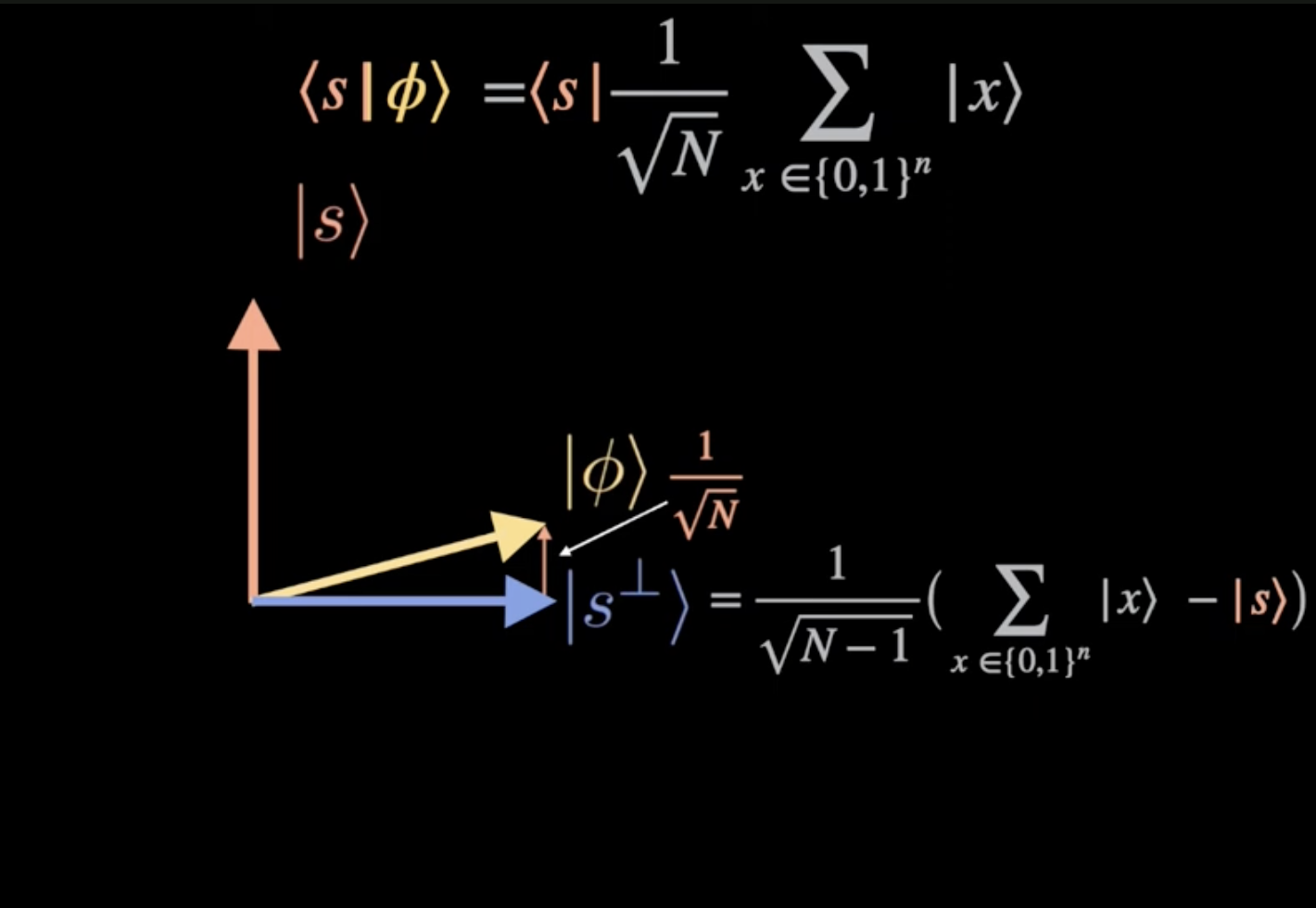
In the visualization above:
- Pink arrow ($\lvert s \rangle$): the solution, pointing vertically
- Blue arrow ($\lvert s^\perp \rangle$): the orthogonal complement, pointing horizontally
- Yellow arrow ($\lvert \phi \rangle$): the initial superposition, at a small angle $\theta$ from horizontal
Composition of Two Reflections
The heart of Grover’s algorithm rests on a lemma from Euclidean geometry that you can verify with the rotation matrices from Calc 3:
Lemma: The composition of two reflections, with angle $\theta$ between their axes, is a rotation by $2\theta$.
If $R_1$ reflects about axis $\ell_1$ and $R_2$ reflects about axis $\ell_2$, and the angle between $\ell_1$ and $\ell_2$ is $\theta$, then $R_2 \circ R_1$ is a rotation by $2\theta$. This is the engine of the algorithm.
Two Reflections = Rotation by \(2\theta\)
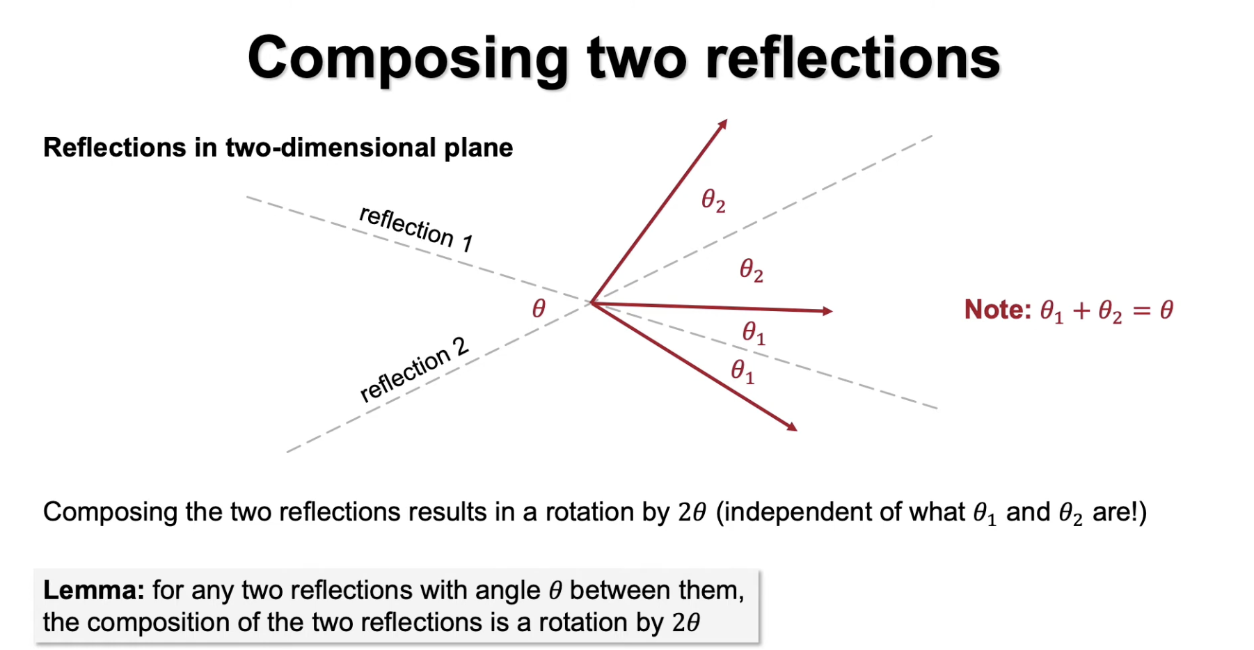
In the diagram: the red vector is reflected to magenta (first reflection), then to purple (second reflection). The net effect? A rotation by $2\theta$. No magic, just geometry.
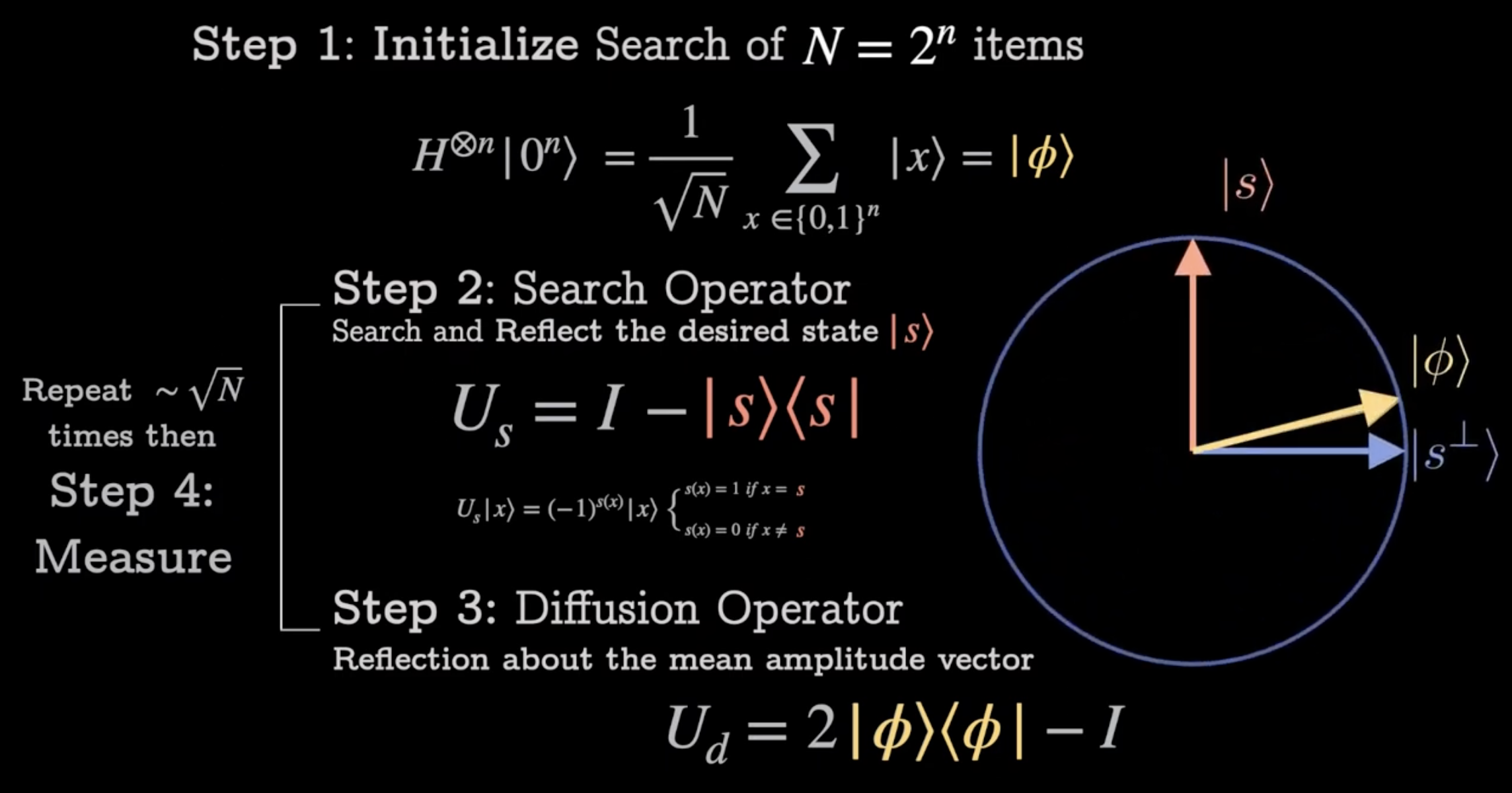
The Grover Iteration
Each iteration of Grover’s algorithm consists of two reflections:
- The Oracle $U_f$: reflects the state about $\lvert s^\perp \rangle$ (flips the sign of the solution component).
- The Diffusion Operator $D = 2\lvert \phi \rangle \langle \phi \rvert - I$: reflects the state about the initial superposition $\lvert \phi \rangle$ (reflects about the mean).
The Grover operator is their composition:
\[G = D \cdot U_f\]By the reflection lemma, $G$ is a rotation by $2\theta$ in the $(\lvert s^\perp \rangle, \lvert s \rangle)$ plane, toward $\lvert s \rangle$. Each application nudges the state vector a little closer to the solution. This is the “small kick” from our calculus bridge.
The Full Procedure
- Initialize: Prepare $\lvert 0 \rangle^{\otimes n}$ and apply $H^{\otimes n}$ to create $\lvert \phi \rangle$.
- Iterate: Apply $G = D \cdot U_f$ a total of $k$ times.
- Measure: Read out the quantum state. With high probability, you get $\lvert s \rangle$.
That is the entire algorithm. Three steps. The rest is understanding why it works and when to stop.
Watch how the purple vector rotates toward the pink solution vector with each iteration. Each step adds $2\theta$ of rotation. The gray horizontal arrow is $\lvert s^\perp \rangle$ for reference.
Now let us see the full analysis with arc trails showing accumulated rotation:
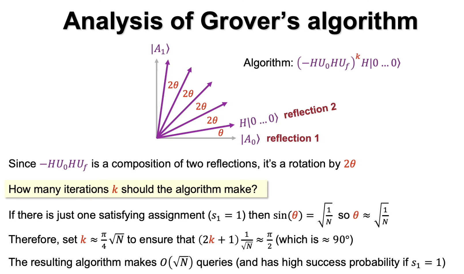
Why $\sqrt{N}$? The Calculus Payoff
Now we cash in the calculus.
After $k$ applications of the Grover operator, the state has been rotated to angle $(2k+1)\theta$ from the $\lvert s^\perp \rangle$ axis. We want this angle to equal $\frac{\pi}{2}$ (pointing straight at $\lvert s \rangle$):
\[(2k+1)\theta = \frac{\pi}{2}\]We know $\sin\theta = \frac{1}{\sqrt{N}}$. For large $N$, $\theta$ is small, and we invoke the Taylor series approximation from Calc 2:
\[\sin\theta = \theta - \frac{\theta^3}{6} + \cdots \approx \theta \quad \text{for small } \theta\]Therefore:
\[\theta \approx \arcsin\!\left(\frac{1}{\sqrt{N}}\right) \approx \frac{1}{\sqrt{N}}\]Substituting:
\[(2k+1) \cdot \frac{1}{\sqrt{N}} \approx \frac{\pi}{2}\] \[k \approx \frac{\pi}{4}\sqrt{N} - \frac{1}{2}\]And there it is: $O(\sqrt{N})$ iterations.
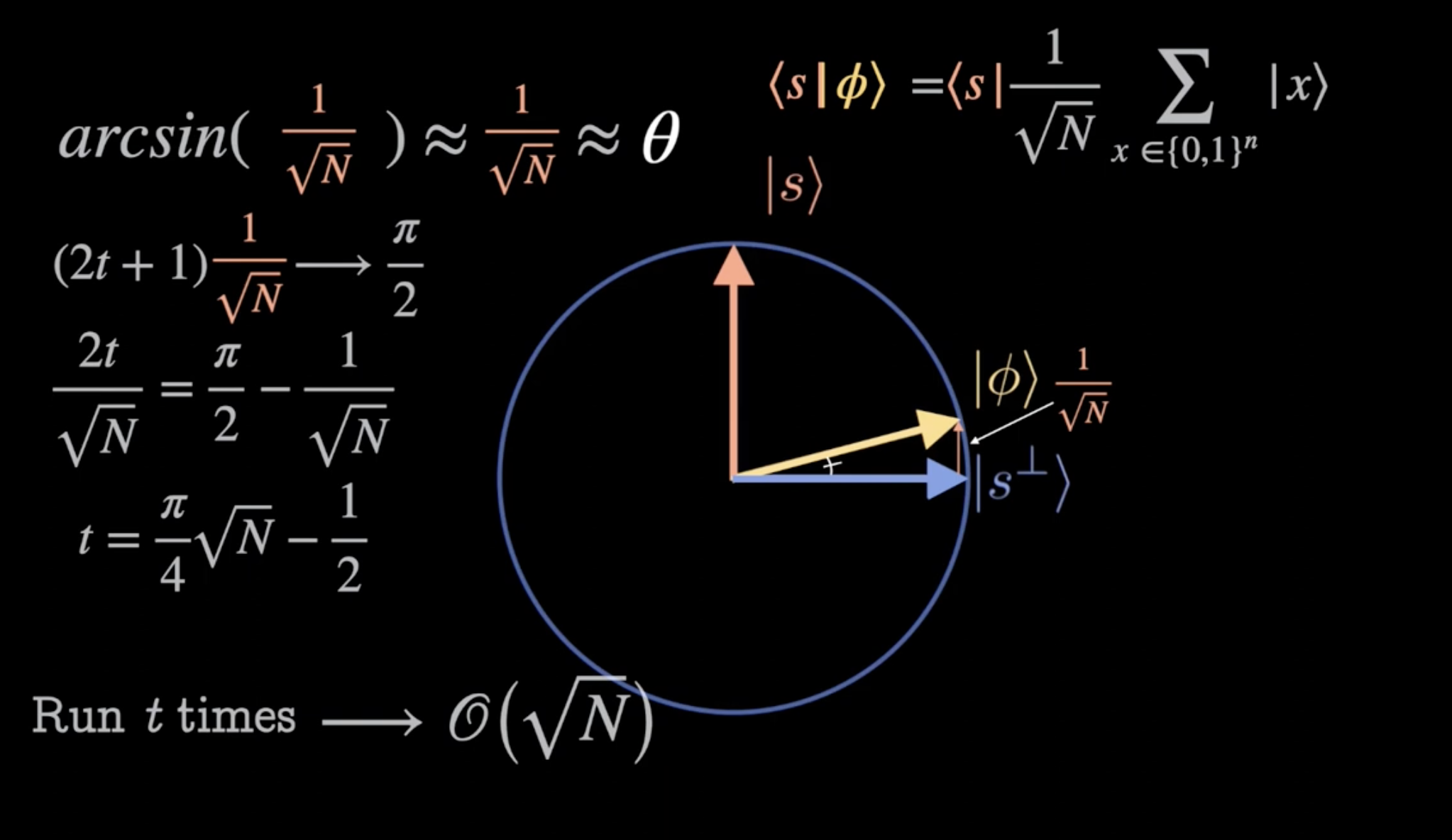
Grover’s algorithm solves unsorted search with $O(\sqrt{N})$ oracle queries – a quadratic speedup over the classical $O(N)$. And Grover proved this is optimal: no quantum algorithm can do better than $\Omega(\sqrt{N})$. The small-angle approximation from your Calc 2 Taylor series is doing real work here.
The Overshoot: Why Grover’s Algorithm Must Be Halted
Now we arrive at the strangest part, and the place where the Euler’s method analogy pays off most beautifully.
In classical search, more work always helps. If you have tried 500 keys and not found the right one, trying 100 more can only improve your situation. You are monotonically narrowing down the possibilities.
Grover’s algorithm is fundamentally different. Running it for too long makes things worse. My God.
The Probability Oscillation
After $k$ iterations of Grover’s algorithm, the probability of measuring the correct answer is:
\[P(k) = \sin^2\!\big((2k+1)\theta\big)\]This is a sinusoidal oscillation. It peaks at $P \approx 1$ when $(2k+1)\theta = \frac{\pi}{2}$, which gives the optimal $k^* \approx \frac{\pi}{4}\sqrt{N}$.
But look at what happens if you keep going:
| Iterations $k$ | Total angle $(2k+1)\theta$ | $P(k) = \sin^2$ | What happens |
|---|---|---|---|
| $0$ | $\theta \approx \frac{1}{\sqrt{N}}$ | $\frac{1}{N}$ | Initial uniform state |
| $\frac{\pi}{8}\sqrt{N}$ | $\frac{\pi}{4}$ | $0.5$ | Halfway there |
| $\frac{\pi}{4}\sqrt{N}$ | $\frac{\pi}{2}$ | $\approx 1$ | Stop here! |
| $\frac{3\pi}{8}\sqrt{N}$ | $\frac{3\pi}{4}$ | $0.5$ | Overshooting… |
| $\frac{\pi}{2}\sqrt{N}$ | $\pi$ | $\approx 0$ | Back to zero! |
The vector has rotated past the solution and is now pointing away from it. Just like Euler’s method overshooting a curve, over-iterating Grover’s sends the state vector past the target. And it keeps going – the probability is periodic, oscillating forever. You had the answer and then you lost it by doing more work. There is no classical analogue to this.
The Grover Overshoot Explorer
Use the sliders below to see this for yourself. Adjust $N$ (database size) and $k$ (iteration count) to watch the state vector move on the unit circle and the probability oscillate.
What to notice (go on, play with it):
- Set $N = 64$ and slowly drag $k$ up. The probability rises to nearly 1 around $k = 6$, then falls back toward 0. You had the answer and kept going.
- Set $N = 1024$ and watch the slower, smoother rise peaking at $k \approx 25$, then the decline.
- The probability is periodic. It will rise again later, but the first peak at $k^* \approx \frac{\pi}{4}\sqrt{N}$ is where you should measure.
This is the deep lesson, and it has no classical analogue: quantum algorithms have a rhythm. Unlike classical computation where more work monotonically improves the result, quantum interference creates oscillations. The art of quantum algorithm design is knowing exactly when to stop. One iteration too many and you start losing what you had.
Recall our Euler’s method analogy: each Grover iteration is a small angular kick of $2\theta$. At the optimal number of kicks, the vector aligns with the answer. One kick too many and you start moving away. The vector swings past $\frac{\pi}{2}$ and the $\sin^2$ probability decreases. The algorithm has overshot. My word.
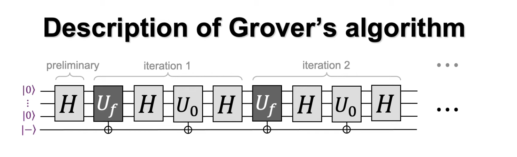
Quantum Circuits
We couch the broader discussion of quantum circuit gates for a future deep dive, but provide a diagram for Grover’s Search for the curious reader who wants to see how the abstract procedure maps to hardware-level operations.
Conclusion
Grover’s algorithm achieves a quadratic speedup for unsorted search: $O(\sqrt{N})$ queries instead of $O(N)$. It does so through a beautiful geometric mechanism – repeated rotations in a two-dimensional subspace – that you can understand entirely through calculus concepts you already possess: small-angle approximations, rotation, and the idea that iterative procedures can overshoot their targets.
Most real-world databases are structured, so the unsorted search problem may seem contrived. But Grover’s algorithm is far more than a database search trick. Its core technique, amplitude amplification, serves as a subroutine in many quantum algorithms, providing quadratic speedups wherever exhaustive search appears as a bottleneck. It is a primitive, not a product.
The Hamiltonian formalism, bra-ket notation, and Hermitian matrices introduced here are the language of quantum computing and quantum mechanics more broadly. As you continue studying, these tools will reappear in quantum error correction, quantum simulation, and the design of new quantum algorithms. We have barely scratched the surface.
For a condensed, hand-written sketch of the derivation based on Nielsen and Chuang, see this PDF.
Sources
Gordan Ma – Grover’s Algorithm Explained (Video)
L. K. Grover. “A fast quantum mechanical algorithm for database search.” Nov. 19, 1996. arXiv: quant-ph/9605043.
M. A. Nielsen and I. L. Chuang. Quantum Computation and Quantum Information. 10th anniversary ed. Cambridge University Press, 2010. ISBN: 978-1-107-00217-3.