Black-Scholes-Merton: I · II · III
A source of noise, a fair game, a distribution that stays positive, and then the formula — from nothing heavier than completing the square.
Vol. I ended with a contract, $(S_T-K)^+$, and a list of assumptions. The price today depends on how $S$ wanders until $T$. This volume builds that wander from coin flips, identifies the distribution it produces, and integrates the payoff against it. The answer is $10.45$.
- Wiener and martingales
- The lognormal, against the normal
- A stock as a lognormal process, and the formula
- Where this goes
1. Wiener and martingales
Two objects: a source of noise, and a notion of a fair game. §3 builds the stock from both.
Wiener process
A Wiener process — also called Brownian motion, written $W_t$ — is the model of pure noise used in this series. Picture a pollen grain on a water surface, or a walker who at every instant takes a tiny random step up or down. The walker’s height at time $t$ is $W_t$.
It is not a stock price. It starts at $0$, it is as likely to be negative as positive, and its typical size at time $t$ is $\sqrt{t}$, not $t$.
Coin-flip construction. Fix a horizon $T$ and chop it into $n$ pieces of length $\Delta t=T/n$. Flip a fair coin at each tick. On heads walk up $\sqrt{\Delta t}$; on tails walk down $\sqrt{\Delta t}$. After time $t=k\,\Delta t$,
\[W_t^{(n)} \;=\; \sqrt{\Delta t}\,(\xi_1+\cdots+\xi_k), \qquad \xi_i=\pm 1 \text{ with equal probability}.\]Each step has mean $0$ and variance $\Delta t$, so $k$ steps have mean $0$ and variance $t$. The CLT says that for large $n$ the position at a fixed $t$ is approximately $\mathcal{N}(0,t)$. Send $n\to\infty$ and the staircase becomes a continuous scribble. That scribble is $W_t$.
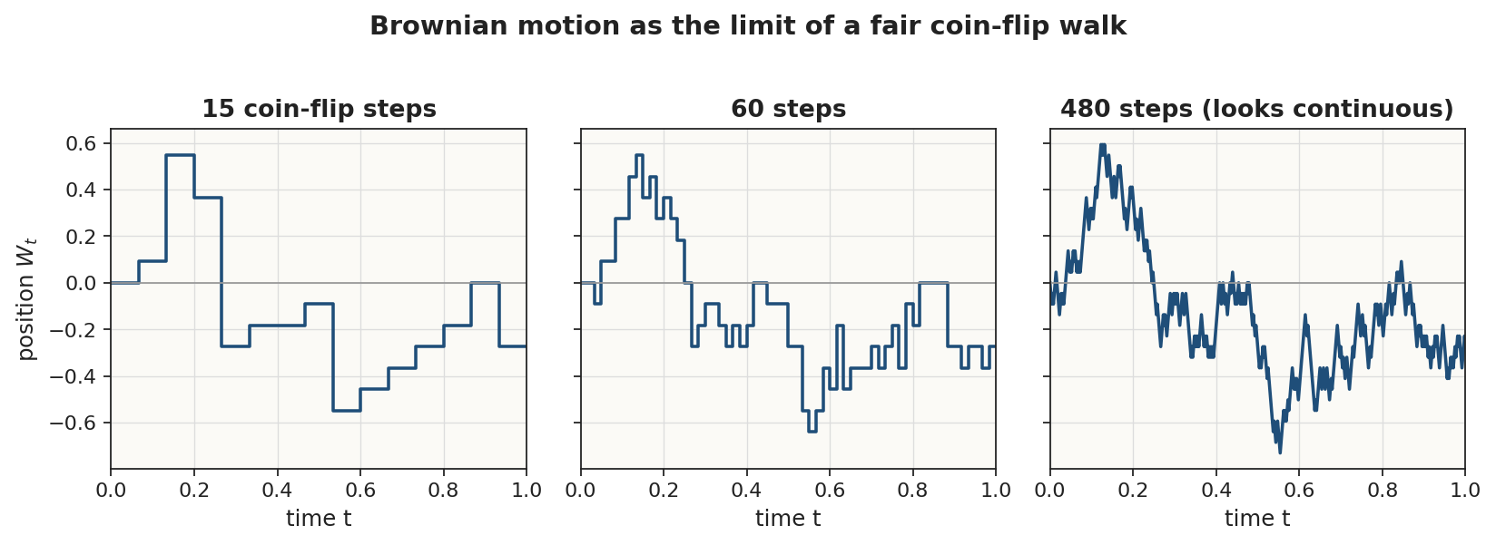
Four properties. A standard Wiener process satisfies:
- $W_0=0$.
- Independent increments. For $t>s$, $W_t-W_s$ does not depend on the path before time $s$.
- Gaussian increments. $W_t-W_s\sim\mathcal{N}(0,\,t-s)$. In particular $W_t\sim\mathcal{N}(0,t)$, so $\mathbb{E}[W_t]=0$ and $\mathrm{Var}(W_t)=t$. The typical size is $\sqrt{t}$. Over a short interval the typical move is $\sqrt{\Delta t}$, much larger than $\Delta t$ when $\Delta t$ is small.
- Continuous paths. No jumps. A jagged scribble with no breaks.
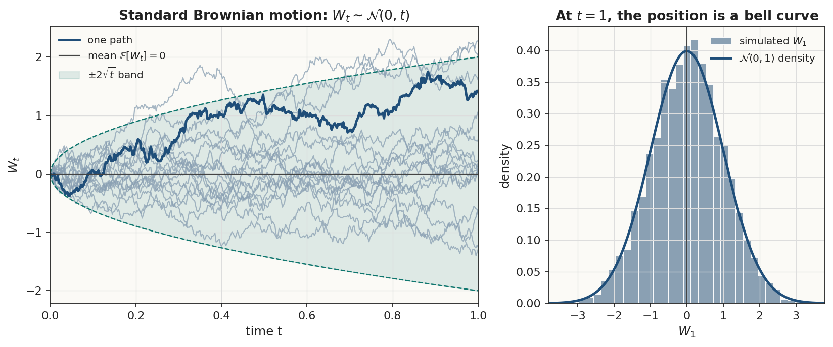
On the left, paths start at $0$ and wander equally above and below — several are negative, which a stock cannot be. The shaded trumpet is $\pm 2\sqrt{t}$. On the right, many runs stopped at $t=1$: the $\mathcal{N}(0,1)$ density.
Write $dW_t$ for an increment over an instant $dt$. Property 3 says $dW_t$ is about $\mathcal{N}(0,dt)$, so $(dW_t)^2$ is typically of size $dt$, not $(dt)^2$. §3 shows why that leftover must be kept. For now, the multiplication table, as a fact about this process:
\[dt\cdot dt \to 0, \qquad dt\cdot dW_t \to 0, \qquad dW_t\cdot dW_t \to dt.\]Martingales
A stochastic process is a family of random variables indexed by time — a random path. A process $M_t$ is a martingale if
\[\mathbb{E}[M_T\mid \text{information up to time }t] \;=\; M_t.\]A martingale is a fair game. Given what you know now, you should not expect to win or to lose.
Wiener itself is a martingale: $\mathbb{E}[W_T\mid W_t]=W_t$, because the remaining increment has mean $0$ and is independent of the past. The physical stock will not be a martingale — it has a drift, which is why anyone bothers to own it. Pricing will live on a different assignment of probabilities, under which the discounted stock is a martingale. That assignment appears in §3, from a two-leaf tree. The definition is here so the word is not magic later.
2. The lognormal, against the normal
Recall the normal
A random variable $X$ is normal with mean $\mu$ and standard deviation $\sigma$, written $X\sim\mathcal{N}(\mu,\sigma^2)$, when its density is
\[\varphi_{\mu,\sigma}(x) \;=\; \frac{1}{\sigma\sqrt{2\pi}}\exp\Bigl(-\frac12\Bigl(\frac{x-\mu}{\sigma}\Bigr)^2\Bigr), \qquad x\in\mathbb{R}.\]The standard normal $Z\sim\mathcal{N}(0,1)$ has density $\varphi(z)=\frac{1}{\sqrt{2\pi}}e^{-z^2/2}$ and cdf
\[\Phi(x) \;=\; P(Z\le x) \;=\; \int_{-\infty}^{x}\varphi(z)\,dz.\]Every normal is a shifted, stretched standard one: $X=\mu+\sigma Z$, so $P(X\le x)=\Phi\bigl((x-\mu)/\sigma\bigr)$. The bell is symmetric about $\mu$, so $\Phi(-x)=1-\Phi(x)$, and the mode, median and mean all sit at $\mu$.
Its lognormal counterpart
Exponentiate: $Y=e^{X}$. Read backwards, $Y$ is lognormal when its logarithm is normal,
\[\ln Y \;\sim\; \mathcal{N}(\mu,\sigma^2).\]Careful with the letters: $\mu$ and $\sigma$ are the mean and standard deviation of $\ln Y$, not of $Y$. Every property of $Y$ is inherited from $X$ by pushing it through $e^x$.
Support. $e^x>0$, so $Y>0$. The normal lives on $(-\infty,\infty)$; the lognormal on $(0,\infty)$.
Median. $e^x$ is increasing, so it preserves order, and order statistics come along for free. The median of $X$ is $\mu$, so the median of $Y$ is $e^{\mu}$.
Mean. Not $e^{\mu}$. The curve $e^x$ bends upward: a swing of $+\sigma$ in $X$ multiplies $Y$ by $e^{\sigma}$, a swing of $-\sigma$ only by $e^{-\sigma}$, and $e^{\sigma}-1>1-e^{-\sigma}$. Symmetric swings in $X$ become lopsided swings in $Y$, and the average is dragged up. By exactly how much is the moment-generating function of $Z$. Completing the square,
\[\mathbb{E}[e^{aZ}] \;=\; \int_{-\infty}^{\infty}\frac{1}{\sqrt{2\pi}}\exp\Bigl(az-\frac{z^2}{2}\Bigr)\,dz \;=\; e^{a^2/2},\]because $az-z^2/2=-\tfrac12(z-a)^2+a^2/2$, and what remains is a normal density with mean $a$, which integrates to $1$. With $Y=e^{\mu}e^{\sigma Z}$ and $a=\sigma$,
\[\mathbb{E}[Y] \;=\; e^{\mu+\sigma^2/2}.\]Variance. The same trick with $a=2\sigma$ gives $\mathbb{E}[Y^2]=e^{2\mu+2\sigma^2}$, so $\mathrm{Var}(Y)=\mathbb{E}[Y^2]-\mathbb{E}[Y]^2=(e^{\sigma^2}-1)\,e^{2\mu+\sigma^2}$.
cdf. $P(Y\le y)=P(X\le\ln y)=\Phi\bigl((\ln y-\mu)/\sigma\bigr)$. Gaussian, in log-coordinates.
Density. Differentiate the cdf, or substitute $x=\ln y$, $dx=dy/y$, into $\varphi_{\mu,\sigma}$:
\[f_Y(y) \;=\; \frac{1}{\sigma\, y\sqrt{2\pi}}\exp\Bigl(-\frac12\Bigl(\frac{\ln y-\mu}{\sigma}\Bigr)^2\Bigr), \qquad y>0.\]Mode. The extra $1/y$ is the Jacobian, and it tilts the peak to the left. Setting the derivative of $\ln f_Y$ to zero gives $e^{\mu-\sigma^2}$.
So where the normal’s three centers coincide, the lognormal’s separate, in a fixed order:
\[\text{mode } e^{\mu-\sigma^2} \;<\; \text{median } e^{\mu} \;<\; \text{mean } e^{\mu+\sigma^2/2}.\]Picture: $\sigma=0.20$, $\mu=\ln 100+0.03$. Mode $\approx 99.0$, median $\approx 103.0$, mean $\approx 105.1$, standard deviation $\approx 21.2$. The most likely neighbourhood is just under $100$; the typical draw lands near $103$; the average is pulled up to $105$ by the right tail. That $e^{\sigma^2/2}$ is Itô’s correction, first as an MGF. §3 recovers it from Taylor.
Side by side
| Normal \(X\sim\mathcal{N}(\mu,\sigma^2)\) | Lognormal \(Y=e^{X}\) | |
|---|---|---|
| arises from | sum of many small pieces | product of many small positive pieces |
| support | \((-\infty,\infty)\) | \((0,\infty)\) |
| shape | symmetric | right-skewed, long upper tail |
| mode / median / mean | \(\mu\) / \(\mu\) / \(\mu\) | \(e^{\mu-\sigma^2}\) / \(e^{\mu}\) / \(e^{\mu+\sigma^2/2}\) |
| variance | \(\sigma^2\) | \((e^{\sigma^2}-1)\,e^{2\mu+\sigma^2}\) |
| closed under | adding independent copies | multiplying independent copies |
| scale by \(c>0\) | scales both \(\mu\) and \(\sigma\) by \(c\) | shifts \(\mu\) by \(\ln c\), keeps \(\sigma\) |
| cdf | \(\Phi\bigl((x-\mu)/\sigma\bigr)\) | \(\Phi\bigl((\ln y-\mu)/\sigma\bigr)\) |
Why a price is lognormal
A stock is a product of returns, not a sum of dollars. Over a day the price multiplies by a gross return $1+R_i>0$. Over $N$ days
\[S_T \;=\; S \prod_{i=1}^{N}(1+R_i), \qquad \ln S_T \;=\; \ln S + \sum_{i=1}^{N}\ln(1+R_i).\]The logs add. If the daily log-returns are independent with finite mean and variance, the CLT says their sum is approximately normal. So $\ln S_T$ is normal, and $S_T$ is lognormal. The normal is what the CLT gives you for a sum of many small independent pieces; the lognormal is what it gives you for a product of many small independent positive pieces. Prices compound, so prices are products.
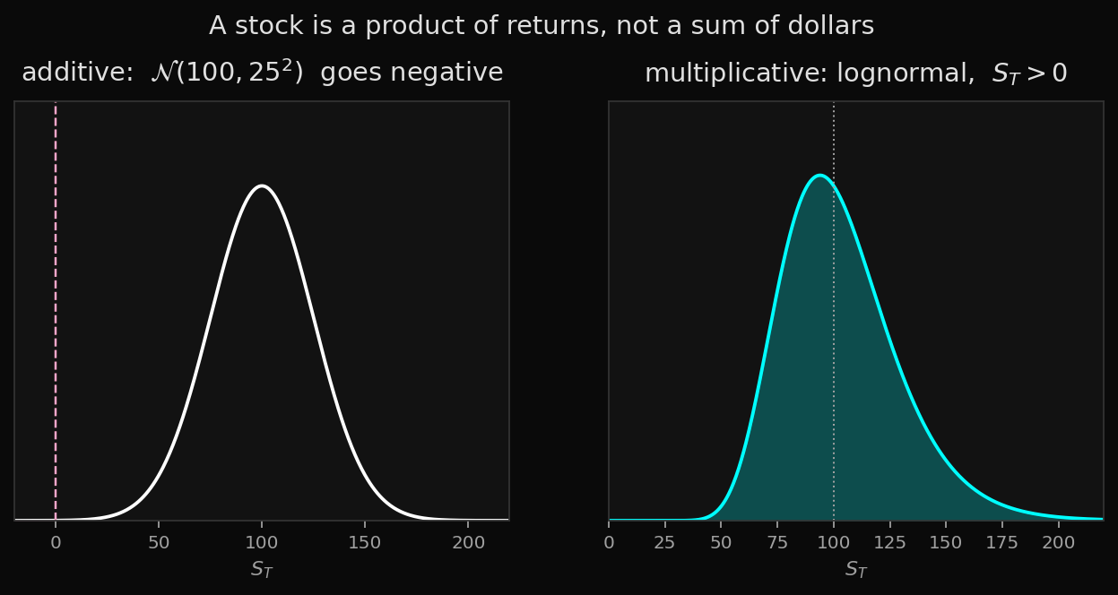
Two objections to a normal for the price are gone. $S_T>0$ always. And a $\$10$ stock and a $\$1000$ stock can share the same $\sigma$, because $\sigma$ measures percentage spread: scaling the price by $c$ just adds $\ln c$ to $\mu$. A normal with a fixed $\sigma$ would give both stocks the same dollar spread, which no one believes.
A change of letters. In §3, $\mu$ and $\sigma$ become the stock’s drift and volatility, and the log-price turns out normal with parameters built from them but not equal to them. To keep the two apart, write the log-price’s parameters as $(m,s)$:
\[\ln S_T \;\sim\; \mathcal{N}(m,s^2),\]and read every fact above with $\mu\to m$, $\sigma\to s$. The mean is $e^{m+s^2/2}$, and $P(S_T\le K)=\Phi\bigl((\ln K-m)/s\bigr)$. The formula in §3 needs nothing else.
3. A stock as a lognormal process
Five steps. Write the stock as an ODE plus noise. Find the one Taylor term that ordinary calculus drops. Use it to show the stock is lognormal and to name $(m,s)$. Integrate the payoff against that lognormal. Then see why the drift $\mu$ must be swapped for the interest rate $r$ — and get the number.
From ODE to SDE
$W_t$ is a bad model for a stock. It can be negative, and a $\$100$ stock and a $\$10$ stock should not make dollar moves of the same typical size.
You already know the ODE $dS=\mu S\,dt$, whose solution is $S_t=S_0 e^{\mu t}$. The model used here is that ODE plus noise, scaled by the current price so the percentage move is Wiener. That is geometric Brownian motion:
\[dS_t \;=\; \mu S_t\,dt + \sigma S_t\,dW_t. \tag{2}\]Read it as a recipe for a short interval $dt$:
- a deterministic fraction $\mu\,dt$ (the drift $\mu$ is the expected rate of return);
- plus a random fraction $\sigma\,dW_t$ (the volatility $\sigma$ scales the Wiener increment).
Because the noise is multiplied by $S_t$, a $\$200$ stock has twice the dollar volatility of a $\$100$ stock, and $S_t$ stays positive. The $d$ on the left is an increment, not a derivative.
A dollar in the money-market account (riskless savings at a constant rate $r$) grows as $B_t=e^{rt}$. Continuous compounding: $e^{0.05}\approx 1.0513$ over a year.
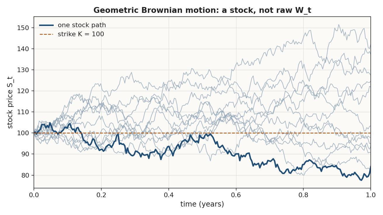
Each path is one draw of $W$, turned into a price by $(2)$. A European call with the dashed strike pays the excess over $100$ if the path ends above the line, and zero otherwise.
The solution of $(2)$ is not $S_0 e^{\mu t}$ times a noise factor. The exponent needs a correction, and the correction comes from a term calculus usually throws away.
The term calculus drops
The chain rule you already know is first-order Taylor. If $x$ moves by $dx$, then $f$ moves by $f’(x)\,dx$, and the next term $\tfrac12 f^{\prime\prime}(x)\,(dx)^2$ is discarded because it vanishes faster than $dx$. For a path with a tangent that discard is legal.
A Wiener path has no tangent. Each increment satisfies $(dW)^2=dt$, the same size as the clock, so the second-order term survives. In 1942 Kiyosi Itô put it back.
Quadratic variation, by hand. Chop a year into four steps. Each step is $\pm\sqrt{1/4}=\pm 1/2$. Four heads ends at $+2$. Four tails ends at $-2$. Mixed paths end at $0$. The ending points disagree. The sum of the squared steps does not:
\[\bigl(\tfrac12\bigr)^2+\bigl(\tfrac12\bigr)^2+\bigl(\tfrac12\bigr)^2+\bigl(\tfrac12\bigr)^2 \;=\; 1\]on every path.
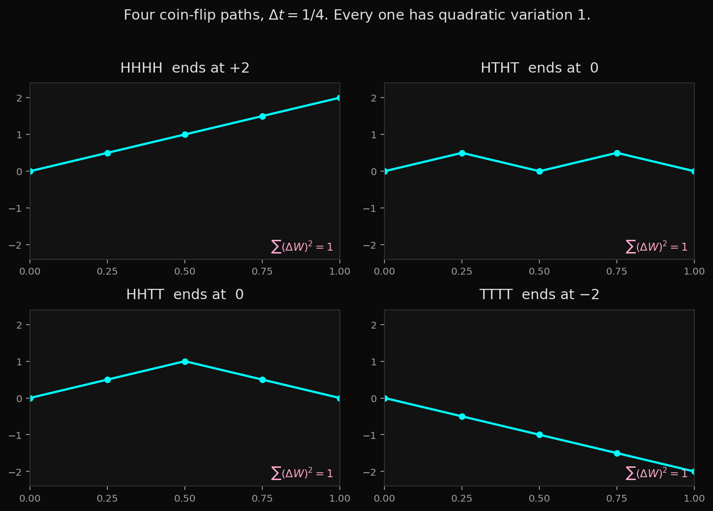
In the limit this is a theorem, and an elementary one. Chop $[0,t]$ into $n$ steps $\Delta t=t/n$. Each increment satisfies $\mathbb{E}[(\Delta W_i)^2]=\Delta t$ and, because $\Delta W_i\sim\mathcal{N}(0,\Delta t)$, $\mathrm{Var}((\Delta W_i)^2)=2(\Delta t)^2$. The sum of squares has mean $t$ and variance $2t^2/n\to 0$. Convergence in $L^2$ to the constant $t$: $(dW_t)^2=dt$. Keep them.
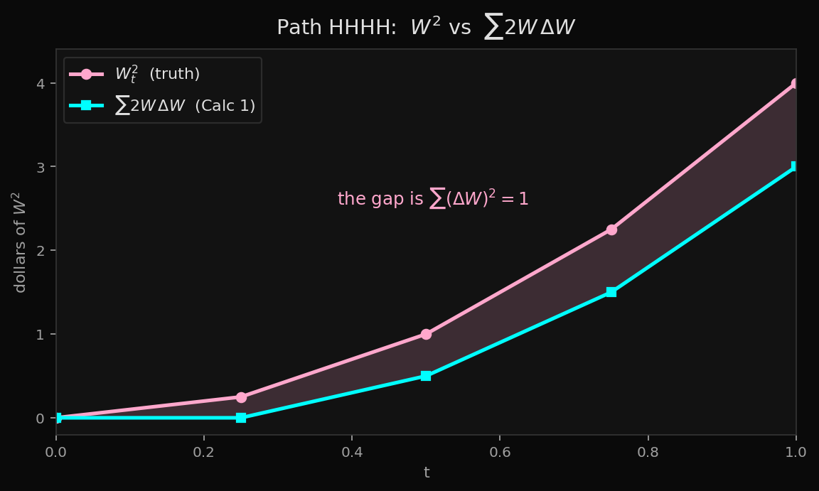
Itô on $W^2$. The chain rule on $f(x)=x^2$ says $\Delta f=2x\,\Delta x$. Taylor keeps the next term $(\Delta x)^2$. On the four-step path of four heads, $W=0,0.5,1,1.5,2$, so $W^2$ ends at $4$. The chain-rule running sum $\sum 2W\,\Delta W$ is
\[2\cdot 0\cdot\tfrac12 + 2\cdot\tfrac12\cdot\tfrac12 + 2\cdot 1\cdot\tfrac12 + 2\cdot\tfrac32\cdot\tfrac12 \;=\; 3.\]The leftover $\sum(\Delta W)^2=1$ makes up the difference: $3+1=4$.
Itô’s lemma is Taylor in two variables, with the multiplication table substituted in. Let $X$ satisfy $dX=a\,dt+b\,dW$, and let $f(t,x)$ be $C^{1,2}$. The second-order expansion is
\[\Delta f \;=\; f_t\,\Delta t + f_x\,\Delta x + \tfrac12 f_{xx}(\Delta x)^2 + f_{tx}\,\Delta t\,\Delta x + \tfrac12 f_{tt}(\Delta t)^2 + o(\Delta t).\]Feed in $\Delta x=a\,\Delta t+b\,\Delta W$. The table kills $(\Delta t)^2$ and $\Delta t\,\Delta W$, and sends $(\Delta x)^2\to b^2\Delta t$. What remains is
\[df(t,X_t) \;=\; \Bigl(f_t + a f_x + \tfrac12 b^2 f_{xx}\Bigr)dt + b f_x\,dW_t. \tag{3}\]The first two terms in the $dt$ coefficient are the ordinary chain rule. The third is the leftover we just computed on $W^2$. For $f(x)=x^2$ and $X=W$ ($a=0$, $b=1$, $f_{xx}=2$), the correction is $dt$, and $d(W^2)=2W\,dW+dt$. At $t=1$ the extra $+1$ is the gap in the figure. This is a derivation by Taylor’s theorem and a check on one path, not a proof in full generality.
The stock is lognormal
Apply $(3)$ to $f(s)=\ln s$ and to the stock $(2)$. Then $f_s=1/s$, $f_{ss}=-1/s^2$, and the leftover is $-\tfrac12\sigma^2\,dt$:
\begin{align}
d\ln S_t
&= \frac{1}{S_t}\,dS_t + \tfrac12\Bigl(-\frac{1}{S_t^2}\Bigr)(\sigma S_t\,dW_t)^2
&= \mu\,dt + \sigma\,dW_t - \tfrac12\sigma^2\,dt
&= \bigl(\mu - \tfrac12\sigma^2\bigr)dt + \sigma\,dW_t.
\end{align}
The right side has constant coefficients, so integrating is just adding. Integrate from $t$ to $T$. Write $\tau=T-t$, and $W_T-W_t\stackrel{d}{=}\sqrt{\tau}\,Z$ with $Z\sim\mathcal{N}(0,1)$:
\[S_T \;=\; S_t\exp\Bigl(\bigl(\mu-\tfrac12\sigma^2\bigr)\tau + \sigma\sqrt{\tau}\,Z\Bigr). \tag{4}\]This is the lognormal of §2, with
\[m \;=\; \ln S_t + \bigl(\mu-\tfrac12\sigma^2\bigr)\tau, \qquad s^2 \;=\; \sigma^2\tau.\]The $\tfrac12\sigma^2$ that left the log-drift is the $e^{s^2/2}$ from the MGF. It returns in the mean of the stock: $\mathbb{E}[S_T\mid S_t]=e^{m+s^2/2}=S_t e^{\mu\tau}$. Nothing is lost. It is booked in a different ledger — the median grows at $\mu-\tfrac12\sigma^2$, the mean at $\mu$.
The call as an integral
Now forget where $(m,s)$ came from. Assume only $\ln S_T\sim\mathcal{N}(m,s^2)$. Split the payoff on $\lbrace S_T>K\rbrace$:
\[\mathbb{E}[(S_T-K)^+] \;=\; \mathbb{E}\bigl[S_T\,1_{\{S_T>K\}}\bigr] - K\,P(S_T>K).\]The second term is the Gaussian tail:
\[P(S_T>K) \;=\; P(\ln S_T>\ln K) \;=\; \Phi\Bigl(\frac{-\ln K+m}{s}\Bigr).\]The first term is a partial expectation: the contribution of the upper tail, not divided by the tail probability. The $x$ in the integrand cancels the $1/x$ in the lognormal density:
\[\mathbb{E}\bigl[S_T\,1_{\{S_T>K\}}\bigr] \;=\; \int_{\ln K}^{\infty}\frac{e^{y}}{s\sqrt{2\pi}}\exp\Bigl(-\frac12\Bigl(\frac{y-m}{s}\Bigr)^2\Bigr)\,dy.\]The exponent is $y-(y-m)^2/(2s^2)$. Expand and complete the square, the same move as $\mathbb{E}[e^{aZ}]$:
\begin{align} y - \frac{(y-m)^2}{2s^2} &= \frac{2s^2 y - (y^2-2my+m^2)}{2s^2} = \frac{-y^2 + 2(m+s^2)y - m^2}{2s^2}. \end{align}
The identity $y^2-2(m+s^2)y=\bigl(y-(m+s^2)\bigr)^2-(m+s^2)^2$ turns the numerator into $-\bigl(y-(m+s^2)\bigr)^2+2ms^2+s^4$. Divide by $2s^2$:
\[y - \frac{(y-m)^2}{2s^2} \;=\; -\frac{\bigl(y-(m+s^2)\bigr)^2}{2s^2} + m + \frac{s^2}{2}.\]The constant $m+s^2/2$ comes out. What remains is a normal density with mean $m+s^2$ and variance $s^2$, truncated at $\ln K$:
\[\mathbb{E}\bigl[S_T\,1_{\{S_T>K\}}\bigr] \;=\; e^{m+s^2/2}\,\Phi\Bigl(\frac{-\ln K+m+s^2}{s}\Bigr). \tag{14}\]The cutoff turned the full MGF factor into that factor times a $\Phi$. The mean-shift $m\mapsto m+s^2$ is the gap between the two $\Phi$ arguments. Combining,
\[\mathbb{E}[(S_T-K)^+] \;=\; e^{m+s^2/2}\,\Phi(d_{+}) - K\,\Phi(d_{-}), \tag{15}\] \[d_{+} \;=\; \frac{-\ln K+m+s^2}{s}, \qquad d_{-} \;=\; \frac{-\ln K+m}{s}.\]If the premium were the discounted expected payoff under this law, it would be $e^{-r\tau}$ times $(15)$. That is the shape of Black–Scholes: two $\Phi$’s, a share piece and a cash piece. What remains is to decide which $m$ to feed it.
Why not $\mu$: a two-leaf tree
The tempting move is to use the physical $m$ from $(4)$, the one with $\mu$ in it. That is wrong, and a cartoon shows why.
A stock trades at $100$. In one year it is either $200$ or $50$. No interest. A call struck at $100$ pays $100$ or $0$.
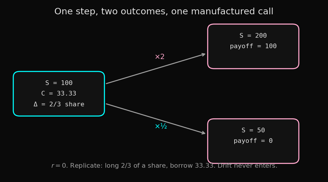
Hold $\Delta$ shares and $B$ dollars in cash (negative $B$ means you borrowed). Match the call on both leaves:
\[200\Delta + B \;=\; 100, \qquad 50\Delta + B \;=\; 0.\]Subtract: $\Delta=2/3$, then $B=-33.33$. Today the portfolio costs $\tfrac23\cdot 100-33.33=33.33$. If the call sold for anything else, you would buy the cheap side and sell the dear side:
| Quote | Today's cash | At expiry |
|---|---|---|
| \(40\) (dear) | sell call, buy portfolio: \(+6.67\) | portfolio covers the call; keep \(6.67\) |
| \(33.33\) | nothing to do | nothing to do |
| \(20\) (cheap) | buy call, sell portfolio: \(+13.33\) | call covers the portfolio; keep \(13.33\) |
A free lunch if the quote is not $33.33$. The physical probability that the stock doubles never entered. Two linear equations.
Now run it backwards. Is there a probability $p^{\ast}$ of the up-move under which the call’s price is simply its expected payoff? Only one makes the stock a fair game — expected value $100$, no drift: $200p^{\ast}+50(1-p^{\ast})=100$, so $p^{\ast}=1/3$. And $C=p^{\ast}\cdot 100=33.33$ again. With interest, a dollar grows by a factor $R$ over the step, the fair-game condition becomes $\mathbb{E}^{\ast}[S_1]=R\,S_0$, i.e. $p^{\ast}=(R-d)/(u-d)$, and the call is the discounted $\mathbb{E}^{\ast}$ of its payoff. That $p^{\ast}$ is not the real-world chance of the up-move. It is the probability that makes the discounted stock a martingale, in the sense of §1. It is called risk-neutral because under it the stock earns only what the bank does.
Notice what changing $p$ to $p^{\ast}$ did not touch: the two leaves, $200$ and $50$. The step sizes set the spread; the probabilities set the drift. That is why $\sigma$ will survive the switch and $\mu$ will not.
A tree calibrated to $r=5\%$, $\sigma=20\%$, one year, $S=K=100$, with Cox–Ross–Rubinstein $u=e^{\sigma\sqrt{\Delta t}}$, $d=1/u$, walks from $12.16$ ($n=1$) to $10.45$ ($n\to\infty$):
| \(n\) | 1 | 2 | 4 | 8 | 16 | 32 | 64 | 128 | \(\infty\) |
|---|---|---|---|---|---|---|---|---|---|
| call | 12.16 | 9.54 | 9.97 | 10.21 | 10.33 | 10.39 | 10.42 | 10.43 | 10.45 |
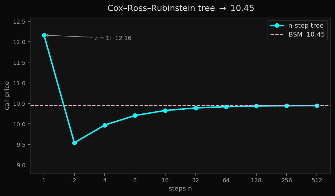
The $n=2$ dip is a coarse histogram of a bell curve. From $n=4$ the walk is toward $10.45$. That is the number. The closed form is the integral $(15)$, with the fair-game $(m,s)$.
Pinning $m$ by elementary statistics
In the limit of the tree, the pricing law is still a lognormal with the same spread $s=\sigma\sqrt{\tau}$ — the leaves did not move — but with the drift chosen so the stock grows, on average, like the bank:
\[\mathbb{E}^*[S_T] \;=\; S_t\,e^{r\tau}.\]That one equation fixes $m$. §2 says the mean of a lognormal is $e^{m+s^2/2}$, so $m+\tfrac12\sigma^2\tau=\ln S_t+r\tau$:
\[m \;=\; \ln S_t + \bigl(r-\tfrac12\sigma^2\bigr)\tau, \qquad s \;=\; \sigma\sqrt{\tau}.\]Equivalently,
\[S_T \;=\; S_t\exp\Bigl(\bigl(r-\tfrac12\sigma^2\bigr)\tau + \sigma\sqrt{\tau}\,Z\Bigr), \qquad Z\sim\mathcal{N}(0,1)\text{ under }\mathbb{Q}, \tag{7}\]which is $(4)$ with $\mu$ replaced by $r$. The letter $\mathbb{Q}$ names this risk-neutral law. The call is its discounted expected payoff:
\[C \;=\; e^{-r\tau}\,\mathbb{E}^{\mathbb{Q}}\bigl[(S_T-K)^+\bigr]. \tag{6}\]The claim that $\sigma$ is untouched, in continuous time, is Girsanov’s theorem; here it is asserted by analogy with the tree, and Vol. III derives it from a ratio of two Gaussian densities. Two traders who disagree about $\mu$ still agree on $C$ if they agree on $\sigma$. $\Delta=2/3$ did not ask who thought the stock would double.
Plug in
Feed the risk-neutral $(m,s)$ into $(15)$. Then $e^{m+s^2/2}=S_t e^{r\tau}$, so the discounted share-piece is $S_t\Phi(d_1)$ and the discounted cash-piece is $K e^{-r\tau}\Phi(d_2)$:
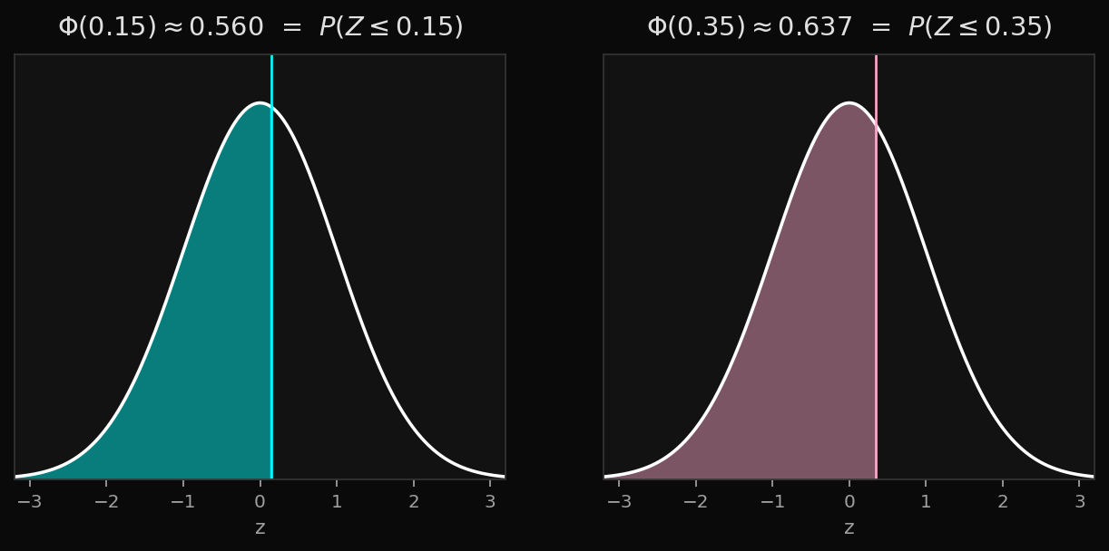
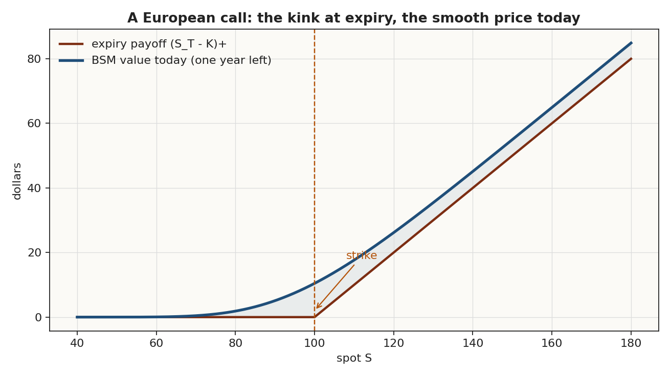
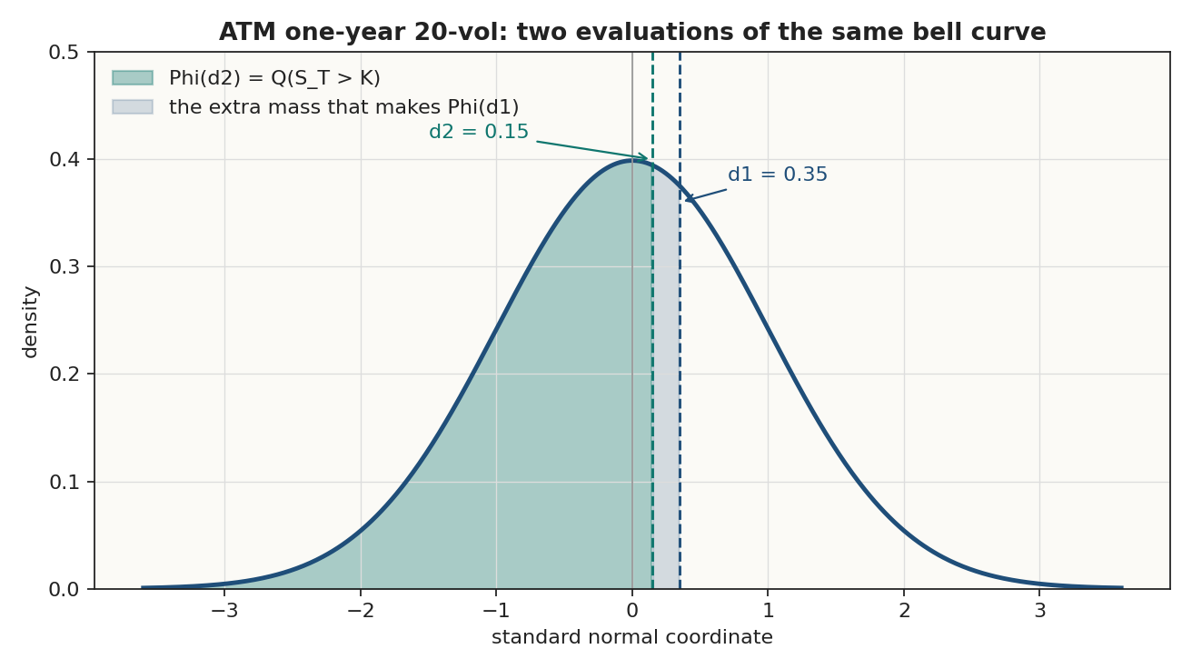
\[C \;=\; S_t\,\Phi(d_1) - K e^{-r\tau}\,\Phi(d_2), \tag{1}\] \[d_1 \;=\; \frac{\ln(S_t/K)+\bigl(r+\tfrac12\sigma^2\bigr)\tau}{\sigma\sqrt{\tau}}, \qquad d_2 \;=\; d_1 - \sigma\sqrt{\tau}.\]That is the Black–Scholes–Merton formula. For the rain check: $S=K=100$, $\tau=1$, $r=0.05$, $\sigma=0.20$. Then $d_2=0.15$, $d_1=0.35$, $\Phi(0.15)\approx 0.560$, $\Phi(0.35)\approx 0.637$, and
\[C \;=\; 100\cdot 0.637 - 100\cdot e^{-0.05}\cdot 0.560 \;\approx\; 63.68-53.23 \;=\; 10.45.\]Vol. I guessed a working premium of $10$. The formula charges $10.45$. Close, for a rain check. $\Phi(d_1)\approx 0.637$ is the delta: you manufacture this call by holding about two-thirds of a share, the $\Delta=2/3$ of the tree, smeared across spots. $\Phi(d_2)\approx 0.560$ is the risk-neutral chance of exercise.
The same arithmetic in Python, standard library only:
from math import log, exp, sqrt, erf

def Phi(x):
    return 0.5 * (1 + erf(x / sqrt(2)))

S, K, r, sig, tau = 100, 100, 0.05, 0.20, 1.0
d1 = (log(S / K) + (r + 0.5 * sig**2) * tau) / (sig * sqrt(tau))
d2 = d1 - sig * sqrt(tau)
C = S * Phi(d1) - K * exp(-r * tau) * Phi(d2)
print(C)  # 10.450583572185565
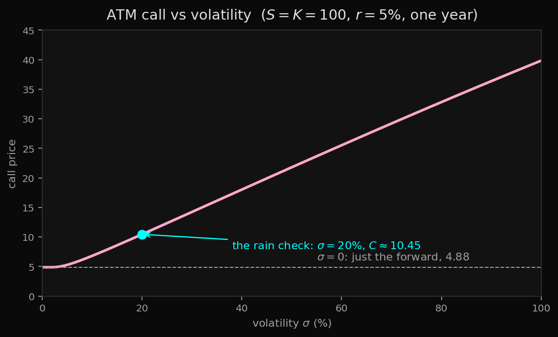
Volatility is the only input you cannot read off a newspaper.
| \(\sigma\) | call | what happened |
|---|---|---|
| \(0\) | \(4.88\) | no wander: just the forward \(S-Ke^{-r\tau}\) |
| \(10\%\) | \(6.80\) | |
| \(20\%\) | \(10.45\) | the rain check |
| \(40\%\) | \(18.02\) | |
| \(100\%\) | \(39.84\) | almost a coin-flip on the stock itself |
Put-call parity. A European call minus a European put, same strike and expiry, is a forward: you will buy the stock at $K$ at time $T$ whether $S_T$ is above or below. A forward on a non-dividend stock is worth $S_t-Ke^{-r\tau}$, so $C-P=S_t-Ke^{-r\tau}$ and
\[P \;=\; K e^{-r\tau}\,\Phi(-d_2) - S_t\,\Phi(-d_1).\]For the rain-check numbers, $P\approx 5.57$, and $C-P=4.88$, the $\sigma=0$ row. That is the accounting identity Vol. I promised for the put.
Where this goes
The derivation used a lognormal, one integral, and a tree. Black and Scholes did not do it this way: they wrote a partial differential equation, and it turns out to be the heat equation in disguise. And the two $\Phi$’s in $(1)$ are probabilities of the same event, $\lbrace S_T>K\rbrace$, yet they differ; a change of numeraire explains why. Those are the first two stops in Vol. III. The third is the list of assumptions from Vol. I, now that we have seen exactly where each one was spent.