Mean-Reverting VIX: I · II · III · IV · V · VI
A model of the VIX is only useful if it prices something you can trade. This volume prices VIX futures and options under the rubber band of Vol. I, reads the futures curve straight out of the option chain, and shows the one thing the simple model cannot do.
Vol. I ended with a model, $d\ln\text{VIX} = \kappa(\theta - \ln\text{VIX})\,dt + \sigma\,dW$, fitted to 22 years of history. History tells you how the VIX moves. It does not tell you what a contract on the VIX costs. For that we need to change worlds.
two worlds: P and Q
The price of a contract that pays $X$ at time $T$ is not $\mathbb E[X]$ under real-world probabilities. If it were, insurance would be priced at its expected loss and nobody would sell it. Investors pay more for payoffs that arrive in bad states of the world, and a VIX call pays off in the worst states of all: when the S&P is falling.
The fundamental theorem of asset pricing packages this into one statement. In a market without arbitrage there is a probability measure $\mathbb Q$ – the risk-neutral or pricing measure – under which the price today of a payoff $X$ at $T$ is
\[\text{price}_t = e^{-r(T-t)}\,\mathbb E^{\mathbb Q}_t[X].\]$\mathbb Q$ is the real-world measure $\mathbb P$ with every outcome re-weighted by how much investors fear it. Under $\mathbb Q$, VIX spikes are more likely than they really are. We keep the form of the model and let its parameters take different values under $\mathbb Q$ than the historical ones of Vol. I. From here until Vol. VI, every parameter is a $\mathbb Q$-parameter, and the only way to learn them is from prices.
VIX futures and the term structure
A VIX future with expiry $T$ settles to $\text{VIX}_T$ (to be exact, to the special opening quotation of the index on the morning of $T$). It costs nothing to enter, so its price $F$ is the number that makes the contract worth zero:
\[F(t,T) = \mathbb E^{\mathbb Q}_t[\text{VIX}_T].\]Under MRLR, $\ln\text{VIX}_T$ is Gaussian (Vol. I) with, writing $\tau = T - t$ and $\phi = e^{-\kappa\tau}$,
\[\mu = \phi\ln\text{VIX}_t + (1-\phi)\,\theta, \qquad v = \frac{\sigma^2}{2\kappa}\,(1-\phi^2).\]For a Gaussian $X\sim\mathcal N(\mu, v)$, $\mathbb E[e^X] = e^{\mu + v/2}$ (complete the square in the Gaussian integral). So
\[F(t,T) = \exp\!\Big(\mu + \tfrac{v}{2}\Big) = \text{VIX}_t^{\,\phi}\;\exp\!\Big(\theta(1-\phi) + \frac{\sigma^2}{4\kappa}\big(1-\phi^2\big)\Big).\]Read it at both ends. For a future about to expire, $\phi\to 1$ and $F\to\text{VIX}_t$. For a distant one, $\phi\to0$ and $F\to e^{\theta + \sigma^2/(4\kappa)}$, a constant: the current VIX stops mattering. Between them the curve bends from spot toward the long-run level. When the VIX is below that level the curve slopes up (contango); after a spike it slopes down (backwardation).
Both happen. On 29 September 2026, with the VIX at 16.04, the curve was in contango. On 26 September 2011, the day Bao’s thesis took its data, the VIX was at 42.3 and the curve was in backwardation. The 2011 futures are not in the thesis; the ones below are what its own calibrated parameters imply (Vol. IV explains how we know).
| spot VIX | VIX futures, first four monthly expiries | ||||
|---|---|---|---|---|---|
| 26 Sep 2011 (thesis parameters) | 42.3 | 37.8–38.5 | 35.0–35.4 | 31.7–32.6 | 32.2–33.4 |
| 29 Sep 2026 (market, via parity) | 16.04 | 17.59 | 18.28 | 18.67 | 19.41 |
the future you cannot build
For a stock, the futures price is pinned by a trade: buy the stock, finance it, deliver it. That gives $F = S\,e^{r\tau}$ (less dividends), the cost-of-carry relation, and it holds because the trade is possible.
For the VIX the trade is impossible (Vol. I: you cannot hold the index). So nothing forces $F = \text{VIX}_t\,e^{r\tau}$, and in fact it fails badly. Whaley (1993), the first VIX option model, treated the index as if it were tradable. On 29 September 2026 that would put the October future at $16.04\,e^{0.0446\times0.0595} = 16.08$. The market says 17.59.
This is why the thesis, and this series, never price VIX options off the spot VIX alone. The model produces $F$ from its dynamics, and the market’s $F$ is a separate, observable number that the model should match. Whether the thesis’ calibration actually matched it is a question for Vol. V.
reading the future out of the option chain
VIX options settle to the same opening quotation as VIX futures. So at expiry a call pays $(\text{VIX}_T - K)^+$ and a put pays $(K-\text{VIX}_T)^+$, and their difference is exactly
\[(x-K)^+ - (K-x)^+ = x - K \quad\text{for every } x.\]Take $\mathbb Q$-expectations and discount with $D = e^{-r\tau}$:
\[C - P = D\,(F - K).\]This is put–call parity, and it holds for any model at all. It is also a measuring instrument. Across every strike where both a call and a put have a live bid, $C-P$ is a straight line in $K$ with slope $-D$ and intercept $DF$. Fitting that line on the full Cboe chain of 29 September 2026 (one rate across the four expiries, least squares) gives
\[r = 4.46\%, \qquad F = 17.59,\ 18.28,\ 18.67,\ 19.41\]for the October, November, December and January expiries. The option chain carries its own futures curve and its own interest rate; we never need a separate futures quote.
VIX options under MRLR
A call is worth $C = D\,\mathbb E^{\mathbb Q}[(\text{VIX}_T - K)^+]$. Under MRLR, $\text{VIX}_T = e^X$ with $X\sim\mathcal N(\mu, v)$ and $e^{\mu+v/2} = F$. The expectation is the same Gaussian integral that produces Black’s formula, and the answer is Black’s formula on the future:
\[C = D\big(F\,\Phi(d_1) - K\,\Phi(d_2)\big), \qquad d_{1} = \frac{\ln(F/K) + v/2}{\sqrt v}, \quad d_2 = d_1 - \sqrt v,\]with $\Phi$ the standard normal CDF. The whole content of mean reversion sits inside two numbers: the level $F$ and the total variance $v = \frac{\sigma^2}{2\kappa}(1-e^{-2\kappa\tau})$.
Keep the shape of this formula. In Vol. III the two normal probabilities $\Phi(d_1)$, $\Phi(d_2)$ become two Fourier integrals, but the structure $D(F\,\Pi_1 - K\,\Pi_2)$ survives.
implied volatility
Prices of options at different strikes are hard to compare by eye. The standard trick converts each price into a single volatility.
The Black price increases with $\sigma$, so the inversion is well defined, and a one-dimensional root-finder solves it. The thesis uses exactly this definition (its Eq. 7.11) with the future as underlying, and warns against the alternative with the spot VIX as underlying and cost-of-carry drift, which manufactures a skew that isn’t there.
Plot implied volatility against strike and you get the smile (or skew) of the market. For S&P 500 options it slopes down: crash puts are expensive. For VIX options it slopes up, because a crash in the S&P is a spike in the VIX, and VIX calls are the crash insurance.
the flat smile
Here is the theorem that motivates the rest of the thesis.
Proof. The MRLR price is Black’s formula with total variance $v$. Setting $\sigma_{\text{imp}}^2\tau = v$ reproduces it at every strike, and the inversion is unique. $\square$
A log-normal model has a flat smile. Now look at the market. Below is the implied volatility of every October 2026 VIX call with a live bid and open interest, against the parity future $F = 17.59$: grey bars are bid-to-ask. (The three lines are the calibrated models of Vol. V; ignore them for now.)
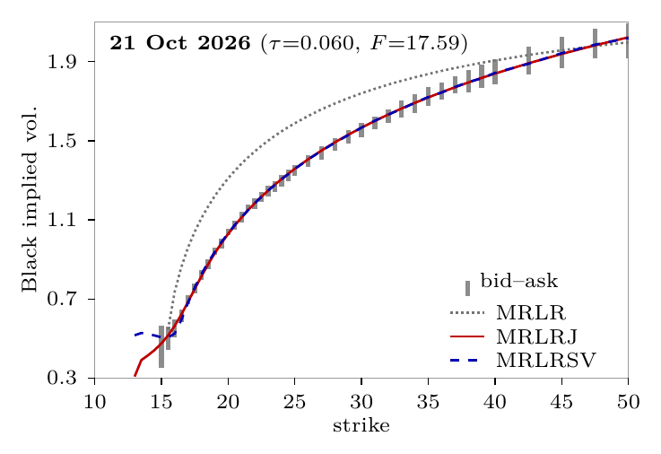
VIX call implied volatility, 21 Oct 2026 expiry, quoted 29 Sep 2026. From about 0.75 at the money to about 2.0 at a strike of 50.
The smile is not flat. It is a wall: implied volatility nearly triples between the money and a strike of 50. Put numbers on it. Take MRLR with its variance set to match the at-the-money option ($\sigma_{\text{imp}} = 0.75$ at $K = 17.5$) and price the out-of-the-money calls:
| strike | market bid / ask | flat-smile (MRLR) price |
|---|---|---|
| 25 | 0.47 / 0.53 | 0.041 |
| 30 | 0.28 / 0.34 | 0.002 |
| 40 | 0.13 / 0.19 | 0.000 |
| 50 | 0.06 / 0.11 | 0.000 |
No choice of $(\kappa, \theta, \sigma)$ fixes this: every choice gives a flat line, and a flat line can match the at-the-money price or the wing prices, never both. Vol. V shows what the best compromise costs: errors of 28–38%, and a model future that lands 27–30% below the market.
where this goes
To bend the smile upward, the distribution of $\ln\text{VIX}_T$ needs a fatter right tail than a Gaussian. There are two natural ways to get one: let the VIX jump, or let its volatility be random. Both destroy the closed-form Black formula, and both are rescued by the same idea from Fourier analysis.
Next: Vol. III: Jumps, Vol-of-Vol and the Fourier Trick
Mean-Reverting VIX: Vol. I · Vol. II · Vol. III · Vol. IV · Vol. V · Vol. VI